7 min to read
Analyzing the NASDAQ with Gaussian Processes
A simple demonstration of a powerful tool.

A while back I worked on a fun project using some of the analysis tools from my PhD to analyze stock prices. Originally we just posted it as a GitHub repo, but I thought it would be fun to also post it here. So here it is! You can find the original repo here.
Introduction
The Gaussian process is a widely used tool in data science. The Gaussian process model is typically used for data smoothing, interpolation, and regression. However, there are other applications of Gaussian processes that make it a very powerful model.
In this project, we show that a Gaussian process can be used to infer accelerations and decelerations in time series data. By analyzing accelerations, we are able to identify periods of time with higher and lower impact. We apply our model to the NASDAQ stock index to identify periods of high and low growth rates, then show that these periods correspond to significant macroeconomic events.
By demonstrating how Gaussian processes can be used to identify economic trends, we hope to highlight the model’s broader potential in analyzing complex time series data.
Methodology
Our goal is to demonstrate how to use the Guassian process to infer second derivatives of time series data, not necessarily to derive the equations. As such we will not go into the details of the derivation of the Gaussian process. However, we will provide a brief overview of the model.
The main assumption of a Gaussian process model is that if we evaluate a function, $F(t)$, at a collection of points, $t_1, t_2, \ldots, t_n$, then the values of the function at these points will be Gaussian distributed
\[\boldsymbol{f} = \mathcal{N}(\boldsymbol{\mu}, \boldsymbol{K})\]where $f_n=F(t_n)$, $\boldsymbol{\mu}$ is the mean vector (which we will set to 0), and $\boldsymbol{K}$ is the covariance matrix. The covariance matrix is defined as
\[K_{ij} = a^2\exp\left(-\frac{(t_i-t_j)^2}{2\ell^2}\right)\]where $a$ is the amplitude of the function, and $\ell$ is the length scale. The amplitude determines the magnitude of the function. The length scale determines how quickly the function changes with respect to time.
In our case our function $F(t)$ tracks the value of NASDAQ stock index at time over time. But, we say “value” we don’t mean the actual stock price, but rather what it is intrinsically worth. We assume the stock price is randomly distributed around the value at each point in time
\[P(y_n) = \mathcal{N}(F(t_n), \sigma^2)\]where $y_n$ is the stock price at time $t_n$, and $\sigma^2$ is the variance of the stock price.
Without getting into the details, which are beyond the scope of this write-up, we can use the stock prices at different times to infer the value of the stock at different times, ${t^}_1, {t^}_2, \ldots, {t^*}_n$. The equation for this is
\[\boldsymbol{f}^* = \boldsymbol{K}^* (\boldsymbol{K} + \sigma^2\boldsymbol{I})^{-1}\boldsymbol{y}\]but this just gives the value of the stock, it doesn’t tell us how much it is changing. To get the acceleration, we need to take the second derivative of the function. The useful part of the Gaussian process is that we can take the second derivative of the function by taking the second derivative of the covariance matrix
\[\boldsymbol{f}^* = (\dfrac{d}{dt}\boldsymbol{K}^*) (\boldsymbol{K} + \sigma^2\boldsymbol{I})^{-1}\boldsymbol{y}\]where
\[\dfrac{d}{dt}K_{ij} = a^2\exp\left(-\frac{(t_i-t_j)^2}{2\ell^2}\right)\left(\frac{(t_i-t_j)}{\ell^2}\right).\]So all in all we have a very simple equation relating the stock prices to the acceleration of the stock prices.
Just a note: in the code we provide, the equations won’t match up exactly with what we have here since we use a slightly different model called a Structured Kernel Interpolation (SKI) model. If you want to know more feel free to check out our previous work on it here.
Results
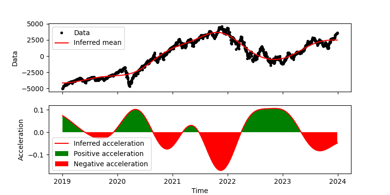
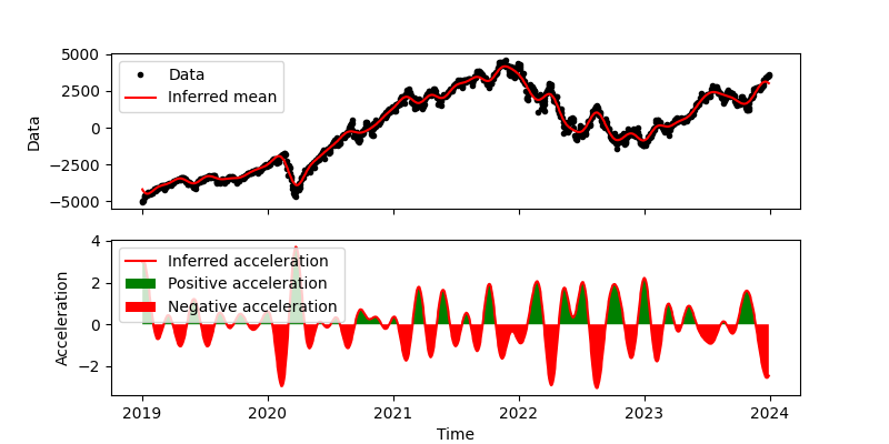
We run our model on the NASDAQ stock index from 2019 to 2024. The results are shown in the figures below. We apply our model using two different length scales, $l=30$ days and $l=180$ days.
We first apply our model with $l=30$ days.
 As you can see, there are clear spikes of acceleration at major turns in the market. At this resolution, however, we see more rapid shifts in the market, so it may be better to choose a length scale that is longer than 30 days.
We then apply our model with $l=180$ days.
 We again see large spikes of acceleration at major turns in the market. However, we see fewer spikes, and the spikes are more pronounced. We will use our results from this model to identify significant macroeconomic events.
Interpretation
We observe the highest accelerations in the NASDAQ’s growth rate around the dates of April 17, 2020, May 5, 2021, and July 25, 2022. Typically, such accelerations follow a period of decline, indicating a local trough in stock prices. These dates coincide with significant macroeconomic events, which are outlined below:
April 17, 2020
- Pandemic Response: The early phase of the COVID-19 pandemic led to global economic disruptions. Markets faced volatility amidst the uncertainty caused by the pandemic.
- Monetary Stimulus: The US Federal Reserve announced a substantial quantitative easing program to inject liquidity into the economy, aiming to mitigate financial stress.
- Fiscal Stimulus: The US Congress passed the CARES Act, providing emergency economic relief to individuals and businesses, which likely had a positive effect on market sentiment.
May 5, 2021
- Economic Recovery: With the progress of covid response campaigns and the lifting of restrictions, economic activities resumed, potentially bolstering technology sectors.
- Accommodative Monetary Policy: The Federal Reserve sustained its low-interest-rate policy and quantitative easing, further supporting the financial markets.
- Corporate Performance: Robust earnings reports from key technology firms, which have a substantial influence on the NASDAQ, likely drove the index higher.
July 25, 2022
- Inflation and Interest Rates: As the Federal Reserve addressed rising inflation through increased interest rates, this led to market adjustments that may have affected growth rates.
- Tech Sector Resilience: Notwithstanding macroeconomic headwinds, the persistent strong performance of technology companies could have buoyed the index.
- Geopolitical Factors: Events such as the conflict in Ukraine introduced additional variables into market dynamics, the implications of which would require specific analysis to understand their impact on the NASDAQ.
In contrast, the highest deceleration in growth rate observed around these dates, August 20th, 2019, November 18th, 2021, and July 7, 2023, do not align with significant socio-economic events as distinctly as the acceleration dates, except for November 29th, 2020 and November 18th, 2021.
November 29, 2020
Market defusing: The NASDAQ at this point was decelerating, possibly as a correction from the rapid growth in the preceding months, as the market adjusted to the new normal of the pandemic. *Election: The US presidential election market a transition of power, which could have introduced uncertainty into the market, leading to a deceleration in growth rates.
November 18, 2021
Inflation Surge: Marking the fastest inflation rate since 1982, energy and food prices saw significant increases, while shelter costs had their highest rise since 2007. Job Growth Disappointment: Despite the sharp fall in the unemployment rate, the economy created far fewer jobs than expected, with notable declines in retail and government employment. Wage Growth: Worker wages continued their upward trend, rising both for the month and significantly over the year.
Conclusion
Here we have shown that Gaussian processes can be used to infer accelerations and decelerations in time series data. We applied our model to the NASDAQ stock index to identify periods of high and low growth rates, then showed that these periods correspond to significant macroeconomic events. By demonstrating how Gaussian processes can be used to identify economic trends, we hope to highlight the model’s broader potential in analyzing complex time series data.
Credits
This work was a joint project between Saivardhan Reddy Ainavolu and Shep Bryan. We hope you enjoyed our work and learned something new. If you have any questions or comments, feel free to reach out to us.


Comments