6 min to read
Comparing different models on biophysics data
A sneak peek into a current project

Here I want to give a sneak peek into a project that my lab is working on. The goal of this project is to compare the results and performance of different deep learning models on a few biophysics datasets. We hope that this will be helpful, giving the community a better understanding of the strengths and weaknesses of different models on biophysics data, so we are structuring the code to be clean and easy to run. You can follow along with the project on GitHub, just please keep in mind that this is a work in progress.
Background
We are looking at three different sets of biophysics data: Bdellovibrio, Retina Vessels, and Fluorescent Neuron Cells. The goal of each dataset is to segment areas of interest.
The first dataset, Bdlellovibrio, is a dataset of phase contrast images of predatory bacteria called Bdellovibrio. These images were captured by our lab and hand annotated (by me, which was an excruciatingly boring process). The goal is to segment the bacteria from the background.
The second dataset, Retina Vessels, is a dataset of retinal images. The goal is to segment the blood vessels from the background.
The third dataset, Fluorescent Neuron Cells, is a dataset of fluorescent images of neuron cells. The goal is to segment the cells from the background.
In the code, we made a simple script, download_data.py, which will automatically download the datasets, clean them, and organize them in the project directory. This way, you can easily run the code on your own machine, knowing that the data you see is the same data we used in the project.
Models
We are comparing four different model architectures: basic Convolutional Network, U-Net, ResNet, and Vision Transformers. While it is common to download pre-built and pre-trained models from the internet, for this project we are building the models from scratch. This also allows the user to see the code for each model and understand how they work. However, keep in mind that because we are applying these models to a specific application, we make choices about model architectures that may be different from standard.
Each model is can be found in the models directory. Each model has the two standard PyTorch Module methods, __init__ and forward, and one nonstandard method called set_output_layer. The set_output_layer method is used to set the number of channels in the output layer of the model. The reason that we do this is so that we can easily experiment with pre-training models as autoencoders and then fine-tuning them for segmentation.
The input to the model is the image and the output is either an image, or class logits, depending on which part of the training we are in. We start by training the model as an autoencoder, then we fine-tune the model for segmentation.
Note that each model has its own parameters that are set during initialization. In addition to comparing models against each other, we will also be comparing the performance of each model with different hyperparameters.
Training and Testing
To ensure that we are robust in our analysis, we use five-fold cross validation for each model we test. That means that for each dataset we look at, we split the data into 5 parts, then run 5 different training and testing sessions, each time using a different part as the validation and test sets. This way, we can be sure that the results we get are not due to random chance.
The functions we use to train and evaluate the model are found in training.py and testing.py. The train_model function takes in a model and a split dataset (split into test, train and validation) then trains the model on the dataset, validating on the validation set, outputting the trained model and the training statistics.
The test_model function takes in a trained model and a test dataset, then evaluates the model on the test dataset, outputting the test statistics. We evaluate the model by looking at the accuracy, sensitivity, specificity, and area under the ROC curve. The ROC curve, which stands for Receiver Operating Characteristic curve, is a plot of the true positive rate against the false positive rate for different thresholds of the class probability. To generate a ROC curve, you calculate logits of each class, convert the logits to probabilities, then vary the threshold of the probability to see how the true positive rate and false positive rate change. You then do that for different values of the threshold from 0 to 1.
Running on HPC
One file in the project, runslurm.sh, is a script that can only be used by our lab. We are keeping the file in the repo in case anyone is curious about how we run our experiments on the ASU High Performance Computing (HPC) cluster.
Results
I want to show some preliminary results for our method here. Just keep in mind that as we test more and more models and hyperparameters, the results may change. In the figure below, we show the segmentation results for each model on the Retina Vessel dataset. The top row shows the input image, the second row shows the ground truth target, and the rest of the rows show the segmentation results for each model.
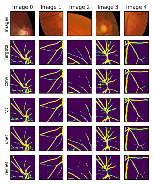
From the figure, we can see that the U-Net model qualitatively performs the best at this segmentation task. The other models have pros and cons, for example the convolutional and resnet capture most of the detail, but have many patches of false positives. The Vision Transformer model has few false positives, but also misses some of the detail.
We can also look at the loss function over time for each model. In the figure below, we show the loss function for each model on the Fluorescent Neuron dataset. We plot the training loss and validation loss in separate panels. For each model, we plot all five folds of the cross validation so we can see how the model performs on different splits of the data.
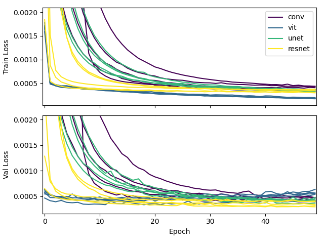
In this figure, you can see that the vision transformer converges to the lowest loss the quickest. The slowest to converge is the convolutional network.
It’s important to note that as we modify the hyperparameters of each model, the results may change.
Conclusion
I hope that you found this sneak peek into our project interesting. I’m excited to see how results change as we compare against different hyperparameters. If you have any questions or comments, please feel free to reach out to me. I’m always happy to talk about my work.


Comments