14 min to read
Dirichlet Clustering for Clinical Outcome Prediction
A simple example

This article is a companion to the GitHub project of the same name. The project contains all the code necessary to run the model described in this article. The code is written in Python and is designed to be easy to read and understand. If you have any questions, please leave a comment below or message me directly.
Introduction
Clustering is an effective way of making predictions. It works by grouping data points together based on their features. Conversely, if we know the cluster a data point belongs to, we can make predictions about it. In medicine, this can be particularly helpful for clinical outcome predictions since, by knowing the cluster a patient belongs to, we can make informed predictions about their diagnosis.
A clustering tool for diagnosis would function as follows: we take a patient, measure various features about them, determine which cluster they most likely belong to, and then make a prediction about their diagnosis based on this cluster. This is a simple yet effective method for predicting a patient’s diagnosis.
However, we cannot deploy this model until we have identified the characteristics of each cluster. Since the cluster that a patient belongs to is often not directly measurable, we must infer the cluster assignments from the data. This is where Bayesian inference comes into play. Bayesian inference is a method of inferring unknown variables from observed data.
In this article, we demonstrate how to build a clustering model using Dirichlet Clustering within a Bayesian framework. We then apply our model to a dataset to predict the diagnoses of patients. We will provide a high-level overview of how the math and the code work, but we won’t dive deep. If you want to delve more into the mathematics behind Dirichlet Clustering, I encourage you to leave a comment below and check out thistextbook.
Data
For this project, we are examining the Pima Indians Diabetes Database from Kaggle. This dataset tracks the medical histories of Pima Indians and their diabetes status.
For each patient, we have eight measured features: Pregnancies, Glucose, Blood Pressure, Skin Thickness, Insulin, BMI (Body Mass Index), Diabetes Pedigree Function, and Age. Additionally, their diabetes diagnosis is indicated in the last column (Outcome). We print the first few lines here:
| Pregnancies | Glucose | BloodPressure | SkinThickness | Insulin | BMI | DiabetesPedigreeFunction | Age | Outcome |
|---|---|---|---|---|---|---|---|---|
| 6 | 148 | 72 | 35 | 0 | 33.6 | 0.627 | 50 | 1 |
| 1 | 85 | 66 | 29 | 0 | 26.6 | 0.351 | 31 | 0 |
| 8 | 183 | 64 | 0 | 0 | 23.3 | 0.672 | 32 | 1 |
| 1 | 89 | 66 | 23 | 94 | 28.1 | 0.167 | 21 | 0 |
| 0 | 137 | 40 | 35 | 168 | 43.1 | 2.288 | 33 | 1 |
For simplicity, we will exclude the Pregnancies column, as its distribution is not well-modeled by a Gaussian. While it could be included in future work using a different distribution, the other features are currently sufficient for our analysis. Additionally, we exclude all rows with missing values, as the treatment of missing data is beyond the scope of this article.
In the main.py file of our GitHub project, we load the data and split it into an 80/20 training and testing set as follows:
# Load data
data = np.genfromtxt('data/diabetes.csv', delimiter=',', skip_header=True)
data = data[:, 1:]                               # Ignore first column (# pregnancies)
data = data[~np.any(data[:, :-1] == 0, axis=1)]  # Filter our rows with missing values

# Split data into training and test sets
np.random.shuffle(data)
split = int(0.8 * data.shape[0])
data_train = data[:split, :]
data_test = data[split:, :]
Now that we have our data we can begin building our model.
Model
Equations
The foundation of any Bayesian model is the mathematical model that supports it. There are two main parts to the model: the equations that give rise to the cluster assignments and the equations that give rise to the measurements. In this section we will derive the equations that support our model.
Cluster Assignments
The foundation of our Bayesian model lies in determining the clustering distributions. To start, we must decide the total number of clusters. Let $K$ be this number, with clusters indexed from $k = 1, …, K$. Now, let $N$ represent the number of patients, indexed from $n = 1, …, N$. Each patient has a cluster assignment $s_n$, where $s_n$ is the cluster that patient $n$ is assigned to, assuming each patient belongs to exactly one cluster. We can represent these assignments as a vector $\mathbf{s} = (s_1, …, s_N)$.
When randomly selecting a patient, they must be assigned to one of the $K$ clusters. Let’s define $\pi_k$ as the probability that a randomly chosen patient is assigned to cluster $k$. In other words, $\pi_k$ represents the proportion of the patient population in cluster $k$. Given that each patient is assigned to one and only one cluster, it follows that the sum of these probabilities must equal one, expressed as $\sum_{k=1}^{K} \pi_k = 1$. This distribution can be represented as a vector $\boldsymbol{\pi} = (\pi_1, …, \pi_K)$.
Measurements
The next part of our model involves defining the feature measurements. Let $F$ be the number of features, indexed with $f=1,…,F$. For each feature, $f$, within each class, $k$, there will be a mean $\mu_{kf}$ and a variance $\sigma_{kf}^{2}$. We can define vectors $\boldsymbol{\mu}$ and $\boldsymbol{\sigma}$ that contain all of the means and variances, respectively.
We differentiate between classes based on their feature variations. Each patient, denoted as $n$, will have one measurement per feature, $f$, which we denote as $x_{nf}$. All of these measurements can be represented as a matrix $\mathbf{X}$, where $\mathbf{X}{nf} = x{nf}$. The probability of a patient having a certain measurement is given by the normal distribution: \(p(x_{nf} | s_n, \boldsymbol{\mu}, \boldsymbol{\sigma}) = \mathcal{N}(x_{nf} | \mu_{s_nf}, \sigma_{s_nf}^{2})\)
In addition to measuring the patients’ features, we also measure their diagnoses. Let $y_n$ represent the diagnosis of patient $n$. The likelihood of patient $n$ having diabetes is conditioned on their class, $s_n$. Each class carries a different diabetes probability. Let $\phi_k$ denote the probability of a patient in class $k$ having diabetes. This can be expressed as a vector $\boldsymbol{\phi} = (\phi_1, …, \phi_K)$. Thus, the probability that a patient has diabetes given their class is: \(p(y_n | s_n, \boldsymbol{\phi}) = \phi_{s_n}^{y_n} (1 - \phi_{s_n})^{1 - y_n}\)
Priors
In the Bayesian paradigm, it’s essential to assign prior distributions to all variables we wish to infer, namely $\boldsymbol{\pi}$, $\boldsymbol{\mu}$, $\boldsymbol{\sigma}$, and $\boldsymbol{\phi}$.
Starting with $\boldsymbol{\pi}$, the Dirichlet distribution is the most appropriate choice. This distribution is ideal for vectors constrained to sum to 1, aligning perfectly with our requirement for $\boldsymbol{\pi}$, where each element represents the proportion of the population in a given cluster. The Dirichlet distribution is parameterized by a vector $\boldsymbol{\alpha} = (\alpha_1, …, \alpha_K)$, with each $\alpha_k$ representing the concentration parameter for cluster $k$. This choice of the Dirichlet distribution for $\boldsymbol{\pi}$ is the reason behind the naming of this method as Dirichlet Clustering.
For the remaining variables, we assign priors as follows: $\boldsymbol{\mu}$ is given a Gaussian prior to reflect our assumption about the distribution of feature means; $\boldsymbol{\sigma}$ is given an inverse gamma prior, a common choice for variance parameters due to its flexibility and conjugacy with the Gaussian distribution; and $\boldsymbol{\phi}$ is given a beta prior, which is a natural choice for modeling probabilities and rates, such as the likelihood of diabetes in each cluster.
Assigning these priors is a crucial step in a Bayesian framework. Priors allow us to integrate prior knowledge or assumptions into our model and, importantly, enable the model to update these beliefs in light of observed data.
Code
The code for this model is available here. I have written the code to be as easy to read and understand as possible. I will provide a high-level overview of the code here, but I encourage you to check out the code for yourself.
Now that we have a mathematical model, we can begin deploying this into code. In model.py, we create a class called DirichletClustering that contains all the code for our model. The class has two main methods: train and predict. The train method takes in the training data and learns the parameters of the model, while the predict method uses the learned parameters to make predictions on the testing data.
One key aspect to pay attention to is how we store the variables from our method. We choose to save these as a Python dictionary object, where each key is the variable name, and each value is its assignment.
  VARIABLES = {
      # Constants
      'n_data': None,             # The number of data entries
      'n_features': None,         # The number of features
      'n_classes': 2,             # The maximum number of classes considered
      # Variables
      'P': None,                  # The probability of the variables
      's': None,                  # The class assignments
      'x': None,                  # The class outcome probabilities
      'mu': None,                 # The feature means
      'sigma': None,              # The feature standard deviations
      'pi': None,                 # The class probabilities
      # Priors
      'x_prior_alpha': .1,        # The x prior alpha
      'x_prior_beta': .1,         # The x prior beta
      'mu_prior_mean': None,      # The mu prior mean
      'mu_prior_std': None,       # The mu prior standard deviation
      'sigma_prior_shape': 2,     # The sigma prior shape
      'sigma_prior_scale': None,  # The sigma prior scale
      'pi_prior_conc': None,    # The beta prior concentration
  }
Notice that we initialize the variables that can be calibrated with None values. For instance, mu_prior_mean represents the mean of the prior distribution for the feature means, which varies for each feature. Our class includes a function initialize_variables that takes in data and then outputs a SimpleNamespace object (similar to but distinct from a dictionary) with initialized variables.
Training and Prediciton
The train method ingests the training data and learns the model’s parameters. This training is accomplished by running a Gibbs sampling algorithm over the data, which iteratively learns the most probable value for each parameter.
In main.py, we start by initializing our model with the desired number of clusters and then executing the training method:
n_classes = 3
model = DirichletClustering(n_classes)
variables, samples = model.train(data_train)
The model learns all the variables, including the state assignments, feature variables, and the probability of outcomes.
The predict function takes in a new dataset and predicts the cluster assignments based on the learned parameters. Our model is designed to ignore features masked with NaN values. For our purpose, which is to predict the diagnosis of the patients, we mask the last column of the data. We then execute the predict function and display the results:
data_test_masked = data_test.copy()
data_test_masked[:, -1] = np.nan
s_pred = model.predict(data_test_masked, variables)
Results
We applied our model to analyze data from the Pima Indians Diabetes Database. Our model was trained on 80% of the data, with the remaining 20% used for testing. We then compared the model’s predicted cluster assignments to the actual cluster assignments.
Our method doesn’t directly predict the patients’ diagnoses. Instead, it predicts the cluster a patient belongs to, and we use these cluster assignments to infer diagnoses. For instance, if a patient is assigned to cluster 1, we predict that they have diabetes with a probability of $\pi_k$.
To evaluate our model’s effectiveness, we compare the predicted probability of diabetes for each cluster, $\phi_k$, with the actual proportion of diabetes diagnoses per cluster. The comparison is illustrated below:
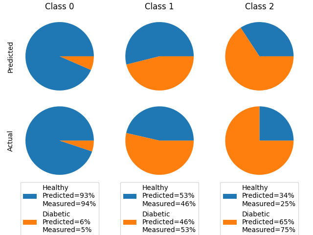
As shown, our model reasonably predicts the probability of diabetes for each cluster, indicating its effectiveness in predicting patient diagnoses.
I would like to add a disclaimer here that we took some shortcuts in the code to make it more readable and easier to run on a typical laptop. You may find that you have to run the script a couple times to obtain the same results as those presented here. This does not mean that the results are random, it just means that the training process is not reaching the same local maximum every time. There are many ways to avoid this issue such as sampling for more iterations or taking ensemble averages instead of point estimates, but we leave this for future work.
Discussion
While this model serves as a robust demonstration, several enhancements would be necessary for real-world deployment. The current iteration provides a foundational understanding, but the complexity of clinical data requires a more nuanced approach. Key areas for improvement include:
-
Dynamic Cluster Number Prediction: Implementing a mechanism to predict the optimal number of clusters based on the data, rather than setting it arbitrarily, would significantly enhance the model’s adaptability and accuracy.
-
Feature Covariance: Incorporating covariance between features can provide a more realistic representation of patient data, as clinical measurements are often interdependent.
-
Non-Gaussian Distributions: Clinical data might not always conform to Gaussian distributions. Exploring non-Gaussian distributions for clusters could allow for more accurate modeling of diverse patient data.
-
Distributions Over Learned Values: Instead of relying on point measurements for learned values, employing distributions offers a more comprehensive view that accounts for uncertainty and variability in the data.
-
Inclusion of Additional Clinical Variables: Incorporating more clinical variables and demographic information could provide a more detailed and accurate clustering.
-
Validation with Larger and Diverse Datasets: To ensure the model’s generalizability and reliability, it should be validated using larger and more diverse datasets from various patient populations.
The primary objective of this article was to highlight the potential of Dirichlet clustering for clinical outcome prediction. It serves as a starting point, offering a glimpse into how Bayesian methods can be applied in a biostatistical context.
Please feel free to dive deeper into the code, build upon it, or adapt it for your own applications. Should you have any questions, insights, or suggestions, please leave me a comment or message. Your feedback is incredibly helpful!


Comments